Dark venues, or pools, are venues in which the players do not see the available liquidity or the limit order book. They started appearing in the past decade after regulatory changes in the US and Europe, like Reg NMS and MIFID, which opened the doors to venue competition. Most importantly, they were made possible by technological advances such as fast communication networks and computational power and their reduced cost and availability. Originally, these pools were designed to allow large orders on opposite sides to trade instantaneously at the primary midpoint, thus avoiding having to split the order into smaller portions and suffering from information leakage. However, dark pools have diverged from their original intent with different pools benefiting different types of traders; some pools are better for large blocks that may take longer to get done, while others o?er a substantial amount of readily available liquidity.
Today, there are about 50 dark pools in the U.S., roughly 20 in Europe and 10 in Asia. They have di?erent rules about minimum order sizes, possible matching prices (midpoint, near touch, far touch), matching rules (time-price priority, price-size priority etc.) and di?erent pricing. Thus the liquidity and microstructure profile of each venue is very different.
How can one optimally route an order to the different dark pools? The objective is a dark aggregation algorithm that goes to most pools and maximizes the amount of liquidity drawn. On average, for relatively large orders, trading in the dark will give slightly lower slippage (when compared to say, a regular lit percent of volume algorithm), but most importantly, dark aggregators allow the investor to have a very high participation without causing too much impact, thus significantly reducing volatility risk. Ideally, we want to post once, get all the liquidity available, and withdraw. This guarantees all executions were at the midpoint with no slippage from subsequent trades. So, the objective is to maximize the amount consumed at a single time step. We use statistics from the Bloomberg Tradebook database to devise a dark aggregator solution that gives a conditional allocation to the amount we are trying to split, giving the aggregator the flexibility to extract the most liquidity from a set of dark pools with a very diverse liquidity profile.
Our motivation for a pure dark allocation algorithm comes from an attempt to answer two questions that are often asked by traders. Suppose we allocated quantity V shares between different venues and received a total of U ≤ V shares. Since we want to maximize U , two questions appear:
- Had we allocated differently, would we have gotten more than U ?
- For a different quantity V , should we allocate to the venues in a similar proportion? In other words, should the weights depend on the allocation size?
The first problem is related to a notion of regret: could we have done better? To understand that, we look at the amount received U . If U = V then there isnt much we could have done. A different allocation would have given us V at best or less at worse. Similarly, if no venue totally consumed the liquidity that was allocated to it, it means we totally consumed the available liquidity, and there isnt much we could have done either. A different allocation would have given us U at best or less at worse.
The second problems answer is intuitively no. We want to maximize the fill ratio of any V we have to allocate, and di?erent venues have di?erent distribution of sizes.
The general idea behind the algorithm is described in Optimal Allocation Strategies for the Dark Pool Problem -that there should be a set a vector weights-one for each total order size we are trying to split. We go over the model and algorithm and simulate the model and the behavior of the allocation algorithm using individual stocks like the LSE stock (London Stock Exchange Group plc trading on the LSE) as well as whole markets (UK and Germany). We use Bloomberg Tradebooks historical trade database to calibrate the model and to simulate the random processes and show graphs of the convergence of the venues weights vectors as a function of the order size. Finally, we discuss the shortcomings of the algo in a posting situation and what type of problem we should really solve in this situation.
RESULTS FOR THE LSE STOCK
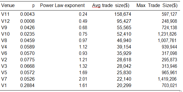
We apply the simulation on the London Stock Exchange Group stock. We have for this stock K = 12. In Table 1, we show the statistics and estimators on the various venues where we traded in 2015: p is the Zero-Bin probability (the probability of going to a venues and not finding any liquidity there), the Power Law exponent is the Pareto tail parameter of the distribution of sizes. We note that the venues with the smallest tail exponent have the highest average trade size, but not always the highest maximum. This is because the maximum is a tail-related statistic, and we have a lot fewer observations on the venues with fatter tails due to their small p. The venue names are hidden and replaced by a numbered series (V1,. . . ,V12). The distributions are estimated, and hence the liquidity profiles of the venues, are very different, which is a perfect application for what we want to achieve.

Table 1: Statistics of venues used for simulation for the LSE stock. Venues are sorted descending by the average trade size.
For instance, notice the estimated shape of the Pareto distribution for V11 is very low (0.24), much lower than any other venue, whereas the probability of getting any fill there is very low (0.43%). V11 is typically a block trading venue where trades are rare but usually of very large size. V1 on the other hand is a very liquid venue but where sizes are typically small. The typical traders we find in V1 would be impatient traders and market makers with small inventory controls trying to supply liquidity or hedge their portfolio often, whereas the typical traders we find in V11 would be large institutional traders with a long term view who are willing to wait for an execution and suffer market volatility risk in favor of large blocks that allow them to minimize information leakage.
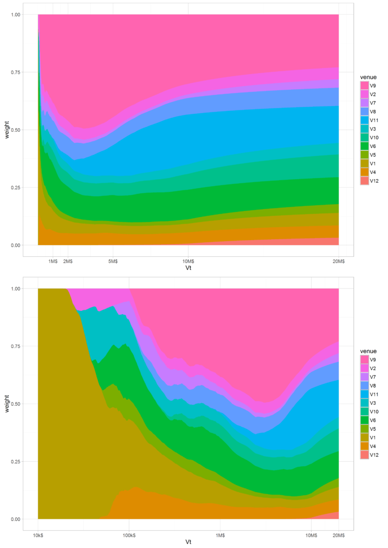
We show the evolution of the weights in time. We see how some venues increase their allocation sizes (and hence weights) under some order sizes, and how they lose out to others under other sizes. We expect then that venues with large tail exponents and high p to dominate the weights when the size of the order is small. This is normal, because when the size to split is small, even a small trade could fully consume the order. Our order would finish sooner if we post on venues like V1 (where p is high). So the determinant of the weight for small sizes is mainly p. As the size to split becomes larger, the tail of the trade sizes becomes more important. Venues with large tail exponents will only give small executions, thus there is no regret in giving them a small size, freeing the remaining quantity to be given to the block venues. The immediate conclusion we make is that the allocation is influenced by both the tail exponent and the Zero-Bin probabilities.
Figure 1 is a map showing the state of the allocation matrix after about 100,000 rounds, after the map has stabilized. The x axis represents the order size we are trying the split and the y axis represents the stacked weights of the various venues, where each venue is represented with a different colour. We see that venues with small tail exponent (fatter tails) will usually have lower fill probabilities and they will dominate the allocation for large order sizes like V9 or V11, but will disappear for small order sizes. Inversely, venues with the largest fill probability like V1 dominate the allocation for small order sizes, but their weight will be small for larger order sizes. Some venues, like V6 and V9, seem to have a wide range of order sizes where they are relevant. For example V6s weights starts gaining importance at the $50k mark and stay relevant all the way to the 20M$ size, whereas V1s weight decreases quickly after the $100k size to reach a very small fraction at the end.

Figure 1: Weights map: for each Vt order size, we show the stacked weights of venues for LN LSE. The x axis on the upper graph is in linear scale and on the bottom graph its in log scale.
RESULTS FOR THE GERMAN MARKET
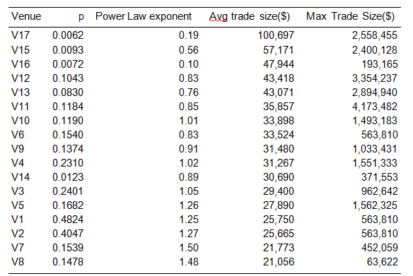
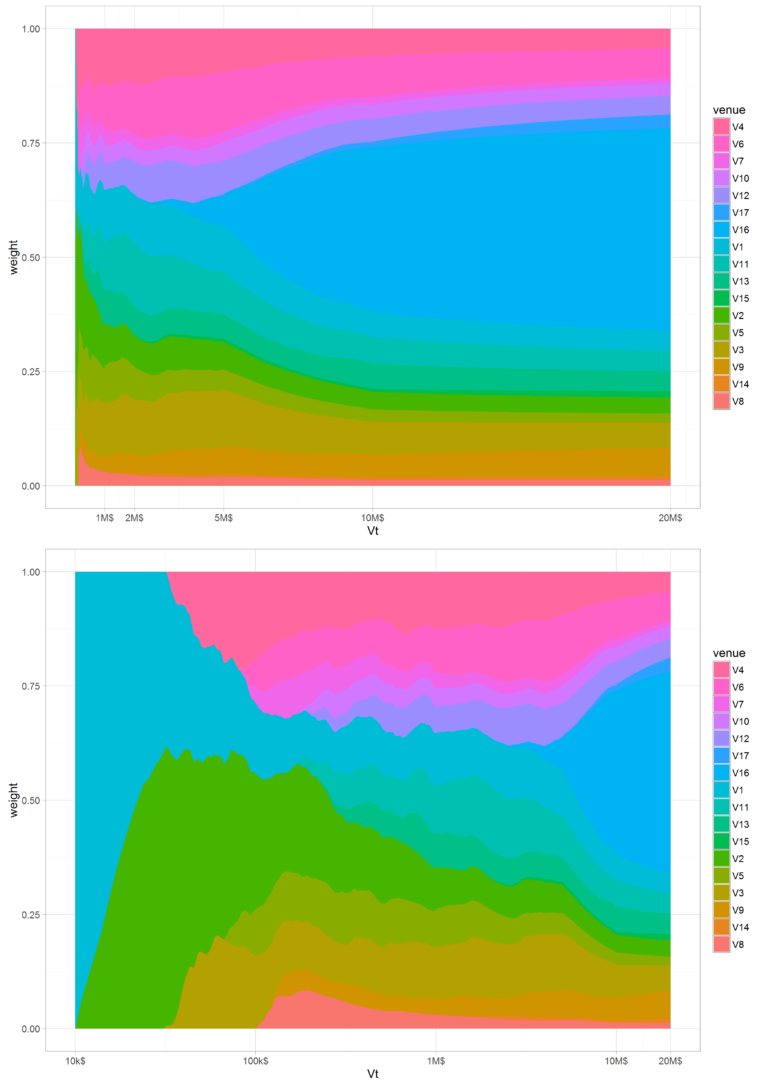
In Germany, there are two block venues, V17 and V16, with a tail exponent of 0.19 and 0.1 respectively (cf Table 2). Figure 2 shows that only V16 manages to acquire a good part of the allocation as the order size increases, becoming quite dominant if the order size is larger than 10M$. When looking at the statistics of both venue, we find this to be normal: the fill probability of V16 = 0.72% is higher than the 0.62% of V17. At the same time, V16 has a fatter tail (α(V 16) = 0.1 < α(V 17) = 0.19). So overall, V16 has liquidity more often and when that liquidity is present, it has a higher probability of being larger. So overall, V16 is a better pool than V17 and the algorithm is right in allocating more to it.

Table 2:Statistics of venues used for simulation over the whole GY market. Venues are sorted descending by the average trade size.

Figure 2: Weights map: for each Vt order size, w7 show the weight of each venue for the whole GY market. The x axis on the upper graph is in linear scale and on the bottom graph its in log scale.
CONCLUSION
We present an algorithm for allocating a parent order between several dark pools. We use the algorithm presented in Optimal Allocation Strategies for the Dark Pool Problem. We simulate the behavior of the algo using estimates based on single stocks as well as markets. The algorithm shows that the allocation should depend on the order size we are trying to split. If the order size is small, give more weights to the most active venues. If the order size is large, then we should give more weight to block venues.


